Lost at the crossroads: genes at the nodes of short-read assembly graphs

5 Mar 2022
metagenomics bioinformatics r

This post is a continuation of my question on Bioinformatics Stack Exchange.

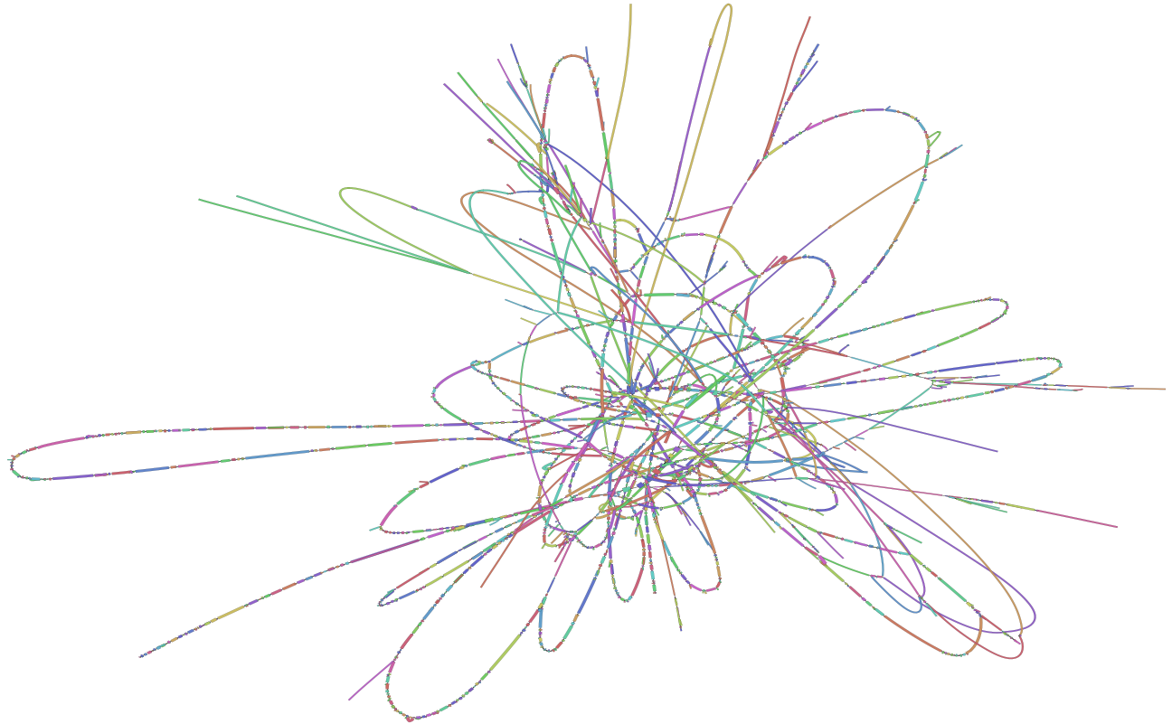
A subset of a Bandage graph for a plasmidSPAdes assembly shows a hairball of segments connected by links

I often use metaSPAdes to assemble short reads from human microbiomes. My simplified understanding of short-read de Bruijn graph assemblers is that they fail where ambiguous paths cannot be resolved. While it can be said that these points of failure may be due to certain structural features of the underlying sequences – long repeats or conserved sequences found at multiple loci – I’m interested in the functional classification of sequences that are proximal to nodes on assembly graphs. Put another way, what kinds of genes are poorly represented in metagenomes because they are poorly assembled? Naively, I expect mobile elements like transposons and integrons to be in such a list of genes, since they are often flanked by repeated sequences and can be present in many copies across multiple genomic contexts, though I want to take an empirical approach.

To that end, I wrote a script to parse assembly graphs in Graphical Fragment Assembly format. Given a GFA file, nodeSeqs.sh will (1) extract segments with at least a minimum number of links, (2) filter those segments given a specified minimum coverage, and (3) trim segment sequences with respect to the orientation of their links. Click the card below to check out the Github repo.

I applied nodeSeqs to six GFA files, each recovered from a human oral microbiome assembly created using ~50 million paired-end reads and default metaSPAdes parameters.

View Code: run nodeSeqs.sh

./nodeSeqs.sh \
  -g assembly_graph_with_scaffolds.gfa \
  -d 5 \
  -c 200 \
  -m 25

Looking at the resulting .fasta files, some of the sequences consist of long stretches of mono- and di-nucleotide repeats, but most of the extracted segments lack any discernible repeat structure. To get at the putative functional roles of these sequences, I ran each sequence set through eggNOG-mapper, which is built to annotate novel sequences using clustered orthologous groups (COGs) of proteins.

View Code: install and run eggNOG-mapper

source /home/miniconda3/bin/activate
conda create --name eggnog-mapper
conda install --channel bioconda eggnog-mapper
conda activate eggnog-mapper

download_eggnog_data.py

# emapper-2.1.7
# Installed eggNOG DB version: 5.0.2
# Diamond version found: diamond version 2.0.14
# MMseqs2 version found: 13.45111

emapper.py \
  -i s1_segments.fasta \
  --itype CDS \
  -m diamond \
  -o s1 \
  --sensmode ultra-sensitive \
  --cpu 8

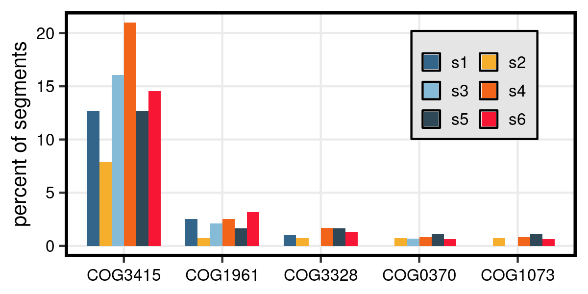
With COG annotations, we can then ask which functions are highly represented among high-degree segments. Plotting the top five functions as proportions of the total number of segments for each sample, we get some interesting results…

View Code: process data and plot results

# clean up annotation headers
sed -i 's/#query/query/g' s*.emapper.annotations

# get total number of segments for each sample, for normalization
for file in ./s*_segments.fasta; do
  num=$(grep -v ">" $file | wc -l)
  echo ${file} | \
  awk -F$'/' '{print $2}' | \
  sed "s/^/${num}\t/g"
done > segment_counts.txt

# process and merge annotation data in the tidyverse
library(tidyverse)
setwd("/workdir/users/acv46/nodeSeqs")

segcounts <- read_tsv("segment_counts.txt", col_names = c("count","sample"))

read_emap <- function(file, segcounts) {
  # file is a list of emapper annotation files
  # segcounts is total segment counts per sample, for normalization
  read_tsv(file = file, comment = "##", col_names = T) %>%
    mutate(sample = str_remove(file, ".emapper.annotations")) %>%
    mutate(totseg = segcounts[which(segcounts$sample == str_remove(file, ".emapper.annotations")),]$count)
}

s1 <- read_emap("s1.emapper.annotations", segcounts)
s2 <- read_emap("s2.emapper.annotations", segcounts)
s3 <- read_emap("s3.emapper.annotations", segcounts)
s4 <- read_emap("s4.emapper.annotations", segcounts)
s5 <- read_emap("s5.emapper.annotations", segcounts)
s6 <- read_emap("s6.emapper.annotations", segcounts)

merge <- bind_rows(s1,s2,s3,s4,s5,s6) %>%
  mutate(COG = sub("@1.*", "", eggNOG_OGs)) %>%
  filter(grepl('COG', COG)) %>%
  select(sample, COG, totseg) %>%
  group_by(sample, COG) %>% mutate(prop = 100*n()/totseg) %>%
  ungroup %>% distinct %>% select(-totseg) %>%
  complete(sample, COG, fill = list(prop = 0)) %>%
  group_by(COG) %>% mutate(avg = median(prop)) %>%
  ungroup %>% arrange(desc(avg))

# get top functions by median across samples
top5 <- merge %>% select(COG, avg) %>%
  unique %>% slice(1:5) %>% select(COG) %>% as_vector

# plot bar graph
pal <- c('#33658a', '#f6ae2d', '#86bbd8', '#f26419', '#2f4858', '#f71735')
ggplot(data = merge %>% filter(COG %in% top5)) +
  geom_bar(mapping = aes(x = factor(COG, level = top5), y = prop, fill = sample),
           stat = "identity", position = "dodge", width = 0.75) +
  theme_bw() +
  scale_fill_manual(values = pal) +
  ylab("percent of segments") +
  theme(axis.title.x = element_blank(),
        axis.title.y = element_text(size = 10),
        axis.text.x = element_text(size = 8, angle = 0,
                                   vjust = 0.5, color = "black"),
        axis.text.y = element_text(size = 8, color = "black"),
        legend.position = c(0.8, 0.7),
        legend.background = element_rect(fill="grey90",
                                  size = 0.5, linetype = "solid", 
                                  colour = "black"),
        legend.text = element_text(size = 8, color = "black"),
        legend.title = element_blank(),
        legend.key.size = unit(3, 'mm'),
        legend.key = element_rect(color = "black"), 
        panel.border = element_rect(color = "black", size = 1.5),
        axis.line.y = element_blank(),
        axis.line.x = element_blank(),
        panel.grid.minor = element_blank(),
        axis.line = element_line(color = "black")) +
  guides(fill = guide_legend(nrow = 3, byrow = TRUE))

Bar graph showing the proportion of high-degree segments from six human oral microbiome assembly graphs that encode proteins which match specific COGs. The 5 COGs with the highest median percentage across samples are shown.

COG3415: Transposase
COG1961: Site-specific DNA recombinase
COG3328: Transposase (or an inactivated derivative)
COG0370: Fe2+ transport system protein B
COG1073: Fermentation-respiration switch protein FrsA

Transposases and recombinases, both common components of mobile elements, are overrepresented at the high-degree junctions of metaSPAdes assembly graphs. This is unsurprising, given the ubiquity of these elements and their sequence conservation across phylogenetic space. The consequence of this is that chromosome-integrated mobile elements are often underrepresented in metagenome-assembled genomes (MAGs). It’s possible that these assemblies could be made better by tweaking the k-mer size, but the greatest potential for improving the contiguity and completeness of MAGs lies in alternative sequencing methods. Long-read sequencing of microbiomes results in more circular contigs and better resolution on the taxonomic associations of the so-called ‘mobilome’. Likewise, proximity ligation sequencing can identify the in situ hosts of plasmids and phage, circumventing the need for association by contiguity.